Semi-automated approaches for interrogating spatial heterogeneity of tissue samples

This notebook is designed to reproduce the main Figures of the manuscript.

from skimage.util import montage
import matplotlib.pyplot as plt
from natsort import natsorted
from anndata import AnnData
import seaborn as sns
import squidpy as sq
import pandas as pd
import scanpy as sc
import numpy as np
import tifffile
import anndata
import zipfile
import copy
import os

# Import helper functions
from utils.utils import *

# Disable warnings
import warnings
warnings.filterwarnings('ignore')

# Disable auto-scrolling
from IPython.display import display, HTML
display(HTML("<style>div.output_scroll { height: auto; max-height: none; }</style>"))
/home/lchen/miniconda3/envs/squidpy/lib/python3.11/site-packages/dask/dataframe/__init__.py:31: FutureWarning: The legacy Dask DataFrame implementation is deprecated and will be removed in a future version. Set the configuration option `dataframe.query-planning` to `True` or None to enable the new Dask Dataframe implementation and silence this warning.
  warnings.warn(
/home/lchen/miniconda3/envs/squidpy/lib/python3.11/site-packages/xarray_schema/__init__.py:1: UserWarning: pkg_resources is deprecated as an API. See https://setuptools.pypa.io/en/latest/pkg_resources.html. The pkg_resources package is slated for removal as early as 2025-11-30. Refrain from using this package or pin to Setuptools<81.
  from pkg_resources import DistributionNotFound, get_distribution
/home/lchen/miniconda3/envs/squidpy/lib/python3.11/site-packages/tqdm/auto.py:21: TqdmWarning: IProgress not found. Please update jupyter and ipywidgets. See https://ipywidgets.readthedocs.io/en/stable/user_install.html
  from .autonotebook import tqdm as notebook_tqdm

Data cleaning

Locate the data

img_path
'data/TMA_downstream_analysis.ome.tiff'
# Path to csv file with single-cell data
file_path ='data/single_cell_dataset.csv'
# Path to image
img_path = r'data/TMA_downstream_analysis.ome.tiff'
# Specify pixel size
px_size = 0.23
# Unzip adata files
for filename in os.listdir( 'data/'):
    if filename.endswith('.zip'):
        with zipfile.ZipFile(os.path.join('data/', filename), 'r') as zip_ref:
            zip_ref.extractall('data/')
# Read the data into a dataframe
data_raw = pd.read_csv(file_path, delimiter = "\t",header=0)
# Randomly shuffle the data frame to make sure all spatial relationships are removed
data = data_raw.sample(frac=1, random_state=42).reset_index(drop=True)
print(data.head(5))
   INDEX Core Tumor type    Sample  Centroid X µm  Centroid Y µm  \
0  55197   B3         PR  Sample 4         2660.2         4091.9   
1  25926   C1        MTX  Sample 1         3644.6         1936.8   
2  39700   G2        MTX  Sample 4         8162.0         3274.0   
3  30747   F1        MTX  Sample 2         7340.0         1868.4   
4  36172   G2        MTX  Sample 4         8118.0         2756.6   

   Detection probability  Nucleus: Area µm^2  Nucleus: Circularity  \
0                 0.9139             23.2439                0.9363   
1                 0.9337             33.9560                0.8777   
2                 0.8549             23.3269                0.4603   
3                 0.9448             59.4584                0.9752   
4                 0.8417             45.2923                0.7699   

   DAPI: Nucleus: Mean  ...  CD8: Nucleus: Mean  PD-1: Cytoplasm: Mean  \
0           11294.1680  ...            802.7551               755.0667   
1           10024.1729  ...            471.7800               675.3105   
2            5785.6074  ...            461.3634               564.8156   
3           17726.8984  ...            487.2480               791.8506   
4            8615.9980  ...            380.3217               746.5083   

   CD4: Nucleus: Mean  PanCK: Cytoplasm: Mean  CD3: Nucleus: Mean  \
0            894.5215                779.1276            463.5465   
1           1182.8143               2312.8086            451.6661   
2            538.6546               2960.0159            204.4086   
3            386.1740              17107.8555            272.1713   
4            936.4126                453.1852            262.2506   

   CD20: Cytoplasm: Mean  CD16: Cytoplasm: Mean  HLA-DR: Cytoplasm: Mean  \
0               547.3238              1768.7448                2912.8591   
1               408.2423               584.5743                6400.9609   
2               429.8794               893.9894                1132.3245   
3               666.1088               504.2844                1528.1755   
4               326.4866               721.8723                8137.2275   

   Vimentin: Cytoplasm: Mean  CD45: Cytoplasm: Mean  
0                  1606.5562               589.1219  
1                  1351.9598               869.6038  
2                  6152.3511               389.6064  
3                  1279.7649               699.5044  
4                  4789.9146               795.5939  

[5 rows x 52 columns]

Perform Leiden clustering and UMAP

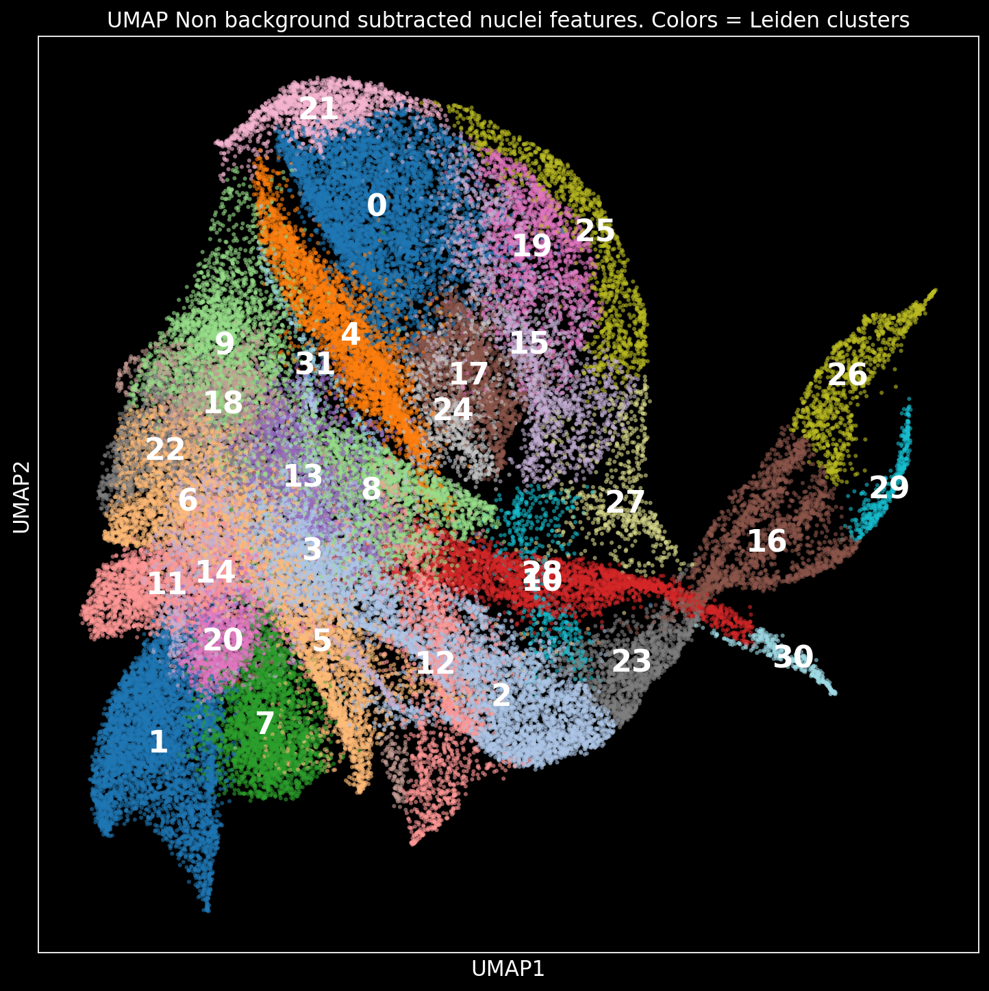
The results of unsupervised clustering an dimensionality reduction using the provided version of scanpy dependency and its sub-dependencies are known to be computer dependent: https://github.com/scverse/scanpy/issues/2014


We provide the unsupervised clustering results that we obtained as a separate AnnData file.
If unsupervised clustring and UMAP is performed using RAW data data, the final results are expected to be different and clsuter names need to be adjusted.

try:
    adata_non_subtracted= anndata.read_h5ad('data/adata_non_substracted.h5ad')
except FileNotFoundError:
    print('No adata_non_subtracted.h5ad file was found. New adata_non_subtracted will be created')
    print('Leiden clustering and UMAP will be performed locally. Results are likely to be different from original manuscript')
    # Get columns for analysis and normalize them
    data_non_subtracted_norm = normalize_median(data.iloc[:, 10:32].to_numpy())
    #Create an AnnData object
    adata_non_subtracted = AnnData(data_non_subtracted_norm,
                                 obsm={"spatial": data[['Centroid X µm', 'Centroid Y µm']].to_numpy()},
                                 obs = {"cores": data['Core'].to_numpy(),
                                        "type": data['Tumor type'].to_numpy()})
    # Change marker names
    adata_non_subtracted.var_names = ['FoxP3','CD68','aSMA','CD31','CD38','IDO1','s100','CD11c','PDL1','Ki67','CD8','PD1','CD4',
                                    'PanCK','CD3','CD20','CD16','HLADR','Vimentin','CD45','Cy5','TRITC']
    
    # Compute neighborhoods
    sc.pp.neighbors(adata_non_subtracted, n_neighbors = 40)
    # Perform leiden clustering
    sc.tl.leiden(adata_non_subtracted, resolution = 1, key_added="RES=1")
    # Perform umap dimensionality reduction
    sc.tl.umap(adata_non_subtracted, min_dist = 0.5)
# Plot clustering results in UMAP coordinates
sc.set_figure_params(figsize='11,11')
plt.style.use('dark_background')
sc.pl.umap(adata_non_subtracted, color="RES=1", title = 'UMAP Non background subtracted nuclei features. Colors = Leiden clusters',  palette = 'tab20', size = 30, alpha =  0.6, legend_fontsize = 20, legend_loc = "on data")

# Plot expression matrix
plt.style.use('default')
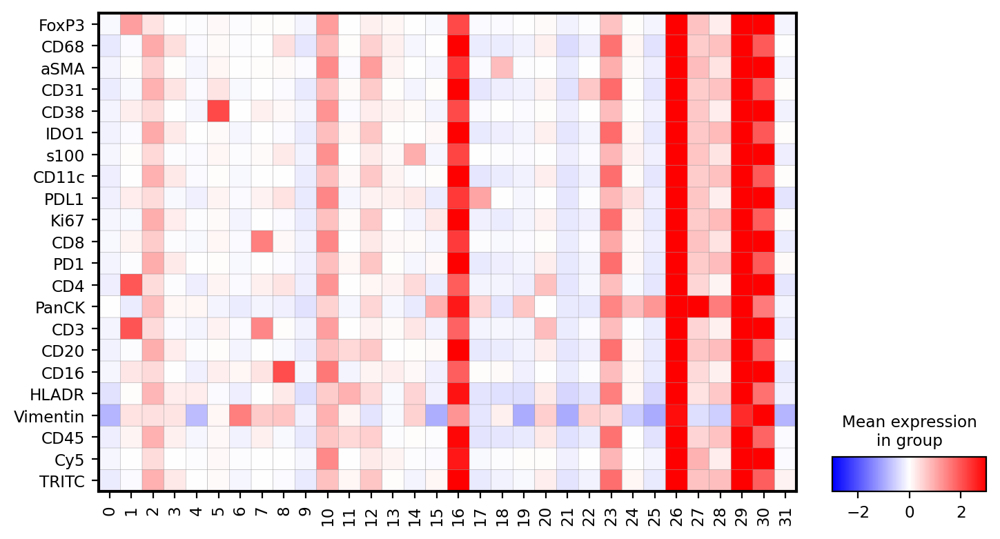
sc.pl.matrixplot(adata_non_subtracted, var_names = adata_non_subtracted.var_names,groupby = 'RES=1',swap_axes = True, figsize = (8.3,4.5), cmap = 'bwr',  vmin = -3, vmax = 3)

Identify clusters with expression over all channels

As discussed in the paper 4 clusters with the highest expression per all markers were identified as mainly composed of erythrocytes.

adata_non_subtracted.X[:3,:4]
print(adata_non_subtracted.X.shape)
(68804, 22)
help(get_sorted_clusters)
Help on function get_sorted_clusters in module utils.utils:

get_sorted_clusters(cluster_names: numpy.ndarray, expression_table: numpy.ndarray)
    Sort the unique cluster names based on the average expression per all markers.
    
    Parameters:
        - cluster_names (numpy.ndarray): Input array containing cluster names [cells]
        - expression_table (numpy.ndarray): Input array containing expression table [cells, markers]
    
    Return:
        tuple [numpy.ndarray, numpy.ndarray] Sorted cluster, sorted av_expression values
bin_mask_erythrocytes
indxs_of_erythrocytes
array([   72,    88,   122, ..., 68757, 68765, 68801], shape=(3432,))
cluster_names = adata_non_subtracted.obs['RES=1'].astype(int)
data_non_subtracted_norm = adata_non_subtracted.X
# Sort clusters based on expression per all markers
sorted_unique_clusters, _ = get_sorted_clusters(cluster_names, data_non_subtracted_norm)
# Take 4 clusters with the highest expression per all markers
err_cluster_names = sorted_unique_clusters[0:4]
# Print clusters of interest
print(f'Identified FP clusters {err_cluster_names}')
# Create a binary mask of erythrocytes
bin_mask_erythrocytes= cluster_names.isin(err_cluster_names).values
# Get the indices of erythrocytes
indxs_of_erythrocytes = np.array([i for i, value in enumerate(cluster_names) if value in err_cluster_names], dtype = int)
Identified FP clusters [26 29 30 16]

Exclude nuclei based on percentile values of:

  • Detection probability > 0.05 percentile
  • DAPI signal mean intensity > 0.05 percentile
  • 0.05 percentile < Nucleus area < 0.999
  • Nucleus circularity > 0.05 percentile


The idea is to exclude the nuclei detections that have low detection probability, are dim, small or very big and non circular.

# Get columns of interest
prob = data['Detection probability'].to_numpy()
DAPI_mean = data['DAPI: Nucleus: Mean'].to_numpy()
area = data['Nucleus: Area µm^2'].to_numpy()
circ = data['Nucleus: Circularity'].to_numpy()

# Define left (q1) and right (q2) percentiles
q1 = 0.05; q2 = 0.999

# Create masks for each condition. Exclude erythrocytes from percentile computation
mask_prob = prob > np.nanquantile(prob[~bin_mask_erythrocytes], q1)
mask_mean = DAPI_mean > np.nanquantile(DAPI_mean[~bin_mask_erythrocytes], q1)
mask_area_smaller = area < np.nanquantile(area[~bin_mask_erythrocytes], q2)
mask_area_larger = area > np.nanquantile(area[~bin_mask_erythrocytes], q1)
mask_circ = circ > np.nanquantile(circ[~bin_mask_erythrocytes], q1)

# Return bitwise AND mask
gating_mask = mask_prob & mask_mean & mask_area_smaller & mask_area_larger & mask_circ
gating_indxs = np.where(gating_mask == 0)[0]

Get original indices for further use and summarize the results

# Get real indices from INDEX column
fp_dapi_cell_indxs = data['INDEX'][gating_indxs].to_numpy()
err_cell_indxs= data['INDEX'][indxs_of_erythrocytes].to_numpy()
# Concatenate indxs all excluded objects
excluded_cell_indxs = np.unique(np.concatenate((fp_dapi_cell_indxs, err_cell_indxs)))

# Printing the numbers of cells excluded
print('GATING_Exclusion. Number of cells: ', len(fp_dapi_cell_indxs))
print('ERYTHROCYTE_Exclusion. Number of cells: ', len(err_cell_indxs))
print('Total number of cells excluded: ', len(excluded_cell_indxs))
GATING_Exclusion. Number of cells:  10797
ERYTHROCYTE_Exclusion. Number of cells:  3432
Total number of cells excluded:  13738

Plot some examples of both types of FPs if image is available

# Only execute this if image is found:
try:
    # Load a DAPI channel from the .ome.tiff image
    DAPI_img = tifffile.imread(img_path, series=0, level=0, key = 0)
    # Specify parameters of CROPS
    img_size_px = 50
    number_of_crops_per_batch = 1000
    normalize_crop = True

    # Get original nuclei coordinates 
    all_nuclei_coords = np.column_stack((data_raw['Centroid X µm'].to_numpy(), data_raw['Centroid Y µm'].to_numpy()))

    # Get coordinates for fp dapi and gated_dapi cells
    gating_coords = all_nuclei_coords[fp_dapi_cell_indxs[0:number_of_crops_per_batch]]
    err_coords = all_nuclei_coords[err_cell_indxs[0:number_of_crops_per_batch]]

    # Get image crops for clusters identified as erythrocytes
    GATING_imgs = get_img_array(DAPI_img, img_size_px, gating_coords, normalize_crop, px_size)
    CLUSTER_imgs = get_img_array(DAPI_img, img_size_px, err_coords, normalize_crop, px_size)

    # Plot montages
    img_count = 16

    # Make montages
    montage_err = montage(CLUSTER_imgs[0:img_count*img_count])
    montage_gating = montage(GATING_imgs[0:img_count*img_count])

    # Cleanup
    del DAPI_img

    # Get centers
    cntr_y = np.repeat(np.arange(img_size_px/2, montage_err.shape[0],img_size_px), img_count)
    cntr_x = np.tile(np.arange(img_size_px/2, montage_err.shape[0], img_size_px), img_count)

    #Plot montages
    fig, ax = plt.subplots(figsize=(15, 15))
    plt.title('Nuclei from excluded clusters (256 random examples)')
    plt.scatter(cntr_y, cntr_x, c = 'yellow', s = 10, marker = 'x')
    plt.axis('off')
    plt.imshow(montage_err, cmap = 'gray', vmin = 0, vmax = 50000)
    plt.show()

    fig, ax = plt.subplots(figsize=(15, 15))
    plt.title('Nuclei excluded by gating (256 random examples)')
    plt.scatter(cntr_y, cntr_x, c = 'yellow', s = 10, marker = 'x')
    plt.axis('off')
    plt.imshow(montage_gating, cmap = 'gray', vmin = 0, vmax = 50000)
    plt.show()
except FileNotFoundError:
    print(f'Image in a specified path {img_path} was not found. Skipping this cell')
Image in a specified path data/TMA_downstream_analysis.ome.tiff was not found. Skipping this cell

Prepare data for phenotyping

print(data_uns.shape)
print(counts_markers_all_norm.shape)
print(len(short_col_names))
print(counts_markers_all.shape)
print(len(core_names_arranged))
(55066, 52)
(55066, 20)
20
(55066, 20)
20
20
#Filter based on data cleaning steps
data_uns = data_raw[data_raw['INDEX'].isin(excluded_cell_indxs) == False]

#Randomly shuffle the data frame
data_uns = data_uns.sample(frac=1, random_state=42).reset_index(drop=True)

# Get all expression data and perform Z-scaling and winsorize
counts_markers_all = data_uns.iloc[:, 32:].to_numpy() # Starting column 32 is cytoplasm
counts_markers_all_norm = normalize_z_scaling(counts_markers_all)
counts_markers_all_norm = winsorize_column_wise(counts_markers_all_norm, [0, 0.0001])

# Short column names
short_col_names = ['FoxP3','CD68','aSMA','CD31','CD38','IDO1','s100','CD11c','PDL1','Ki67',
                   'CD8','PD1','CD4', 'PanCK','CD3','CD20','CD16','HLADR','Vimentin','CD45']

#Create an AnnData object
adata_phenotyping = AnnData(counts_markers_all_norm,
                             obsm={"spatial": data_uns[['Centroid X µm', 'Centroid Y µm']].to_numpy()},
                             obs = {"cores": data_uns['Core'].to_numpy(),
                                    "type": data_uns['Tumor type'].to_numpy(),
                                    'samples': data_uns['Sample'].to_numpy()})
# Change marker names
adata_phenotyping.var_names = short_col_names

# Specify the names that will be used for core arrangement later
core_names_arranged = ['B1','F1','C2','G2','D3','C1','G1','D2','A3','E3','D1','A2','E2','B3','F3','E1','B2','F2','C3','G3']
data_uns.columns[30:36]
Index(['NON_SUBTRACTED_Cy5_Af: Nucleus: Mean',
       'NON_SUBTRACTED_TRITC_Af: Nucleus: Mean', 'FoxP3: Nucleus: Mean',
       'CD68: Cytoplasm: Mean', 'aSMA: Cytoplasm: Mean',
       'CD31: Cytoplasm: Mean'],
      dtype='str')
#help(normalize_z_scaling)
help(winsorize_column_wise)
Help on function winsorize_column_wise in module utils.utils:

winsorize_column_wise(markers_counts: numpy.ndarray, limits: list = None) -> numpy.ndarray
    Winsorize each column of the input array using provided percentiles.
    
    Parameters:
        - markers_counts (numpy.ndarray): Input array containing marker counts.
        - limits (list): limits to be used for winsorization
    
    Returns:
        - numpy.ndarray: Winsorized array.

Supervised phenotyping (Figure 3)

Automatically threshold each marker

2 assumptions are made here: * The first peak of the histogram to the left is a background signal. * Background signal is normally distributed.

adata_phenotyping
AnnData object with n_obs × n_vars = 55066 × 20
    obs: 'cores', 'type', 'samples'
    obsm: 'spatial'
In spatial proteomics workflows (like those for Lunaphore COMET), get_binary_cells is a digitization function. It transforms continuous fluorescence intensity values into a binary "Positive (1) or Negative (0)" matrix.
This is the bridge between raw data (numbers) and biological classification (labels).


help(get_binary_cells)
Help on function get_binary_cells in module utils.utils:

get_binary_cells(z_norm_data: numpy.ndarray, peak_range: tuple = None, sigma_mult: float = 1.0) -> numpy.ndarray
    Generate a binary matrix indicating cells that are positive
    
    Parameters:
        - z_norm_data (numpy.ndarray): 2D array of normalized expression values (markers x cells).
        - peak_range (tuple): Range of the histogram to be used for a peak search.
        - sigma_mult (float): Multiplier for computed background sigma value.
    
    
    Returns:
        - numpy.ndarray: Binary matrix indicating cells that are positive.
# Prepare parameters for marker thresholding
histogram_range = (np.min(counts_markers_all_norm), np.max(counts_markers_all_norm)/5)
# In this paper we used 6 sigma threshold, but it can be adjusted based on the data
sigma_multiplier = 6.0
thresholded_marker_table = get_binary_cells(counts_markers_all_norm, histogram_range, sigma_multiplier)

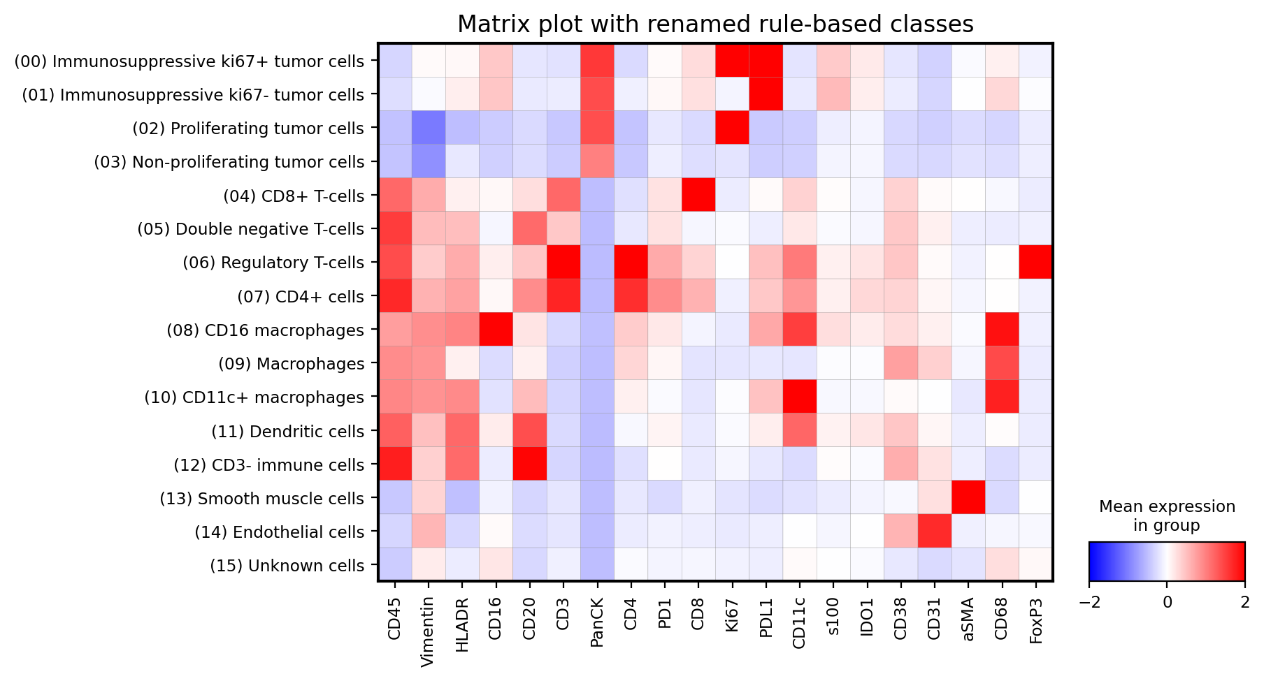
Perform rule based classification

The Classification Logic (The "Tree")  
Here is the breakdown of the logic, translated into biological cell types:  
Level 1: Is it a Tumor Cell? (PanCK+)  
If the cell is PanCK positive, it is an epithelial/tumor cell. The code then checks for activity and evasion:  
    1: Proliferating & Evasive Tumor (PDL1+, Ki67+)  
    2: Evasive Tumor (PDL1+, Ki67-)  
    3: Proliferating Tumor (PDL1-, Ki67+)  
    4: Quiescent Tumor (PDL1-, Ki67-)  
Level 2: Is it an Immune Cell? (PanCK- / CD45+)  
If it's not a tumor cell but is CD45 positive, it’s a leukocyte. It then splits into Lymphoid vs Myeloid:  
T-Cell Lineage (CD3+):  
    5: Cytotoxic T-cell (CD8+)  
    6: Other T-cell (likely CD8- CD4-)  
    7: Regulatory T-cell / Treg (CD4+, FoxP3+)  
    8: Helper T-cell (CD4+, FoxP3-)  
Myeloid Lineage (CD3-):  
    9: Pro-inflammatory/Active Macrophage (CD68+, CD16+)  
    10: Standard Macrophage (CD68+, CD11c-)  
    11: Dendritic-like Macrophage (CD68+, CD11c+)  
    12: Conventional Dendritic Cell / APC (CD68-, HLADR+, CD11c+)  
    13: Other Immune (CD45+ but matches no sub-criteria)  
Level 3: Is it Structural/Stroma? (PanCK- / CD45-)  
If the cell is neither tumor nor immune, it checks for the "infrastructure" of the tissue:  
    14: Fibroblast / Myofibroblast (aSMA+)  
    15: Endothelial Cell / Blood Vessel (CD31+)  
    16: Unclassified / "Other" (The "Dark Matter" of the tissue)  

Why use this specific order? (Hierarchical Bias)  
This code uses a "Mutual Exclusivity" strategy.  
PanCK is First: This is because tumor cells sometimes "gobble up" immune markers or have high background. By putting if cell['PanCK'] at the very top, the code ensures that if a cell is a tumor cell, it stays a tumor cell, even if it has a little bit of "leaky" CD45 signal.  
CD3 before CD68: It defines the adaptive immune system (T-cells) before defining the innate system (Macrophages).  
The "else 16": Every single object in your CSV gets a number. If it doesn't meet any criteria, it becomes a 16. High numbers of "16s" usually suggest your 6-sigma threshold was too strict or you are missing a marker for a specific cell type (like B-cells or NK-cells).  
Summary Table for Mapping  
After running this function, you would typically map these integers back to names:  
ID  Cell Type Name  Primary Marker  
1-4 Tumor           PanCK  
5   CD8 T-cell      CD3, CD8  
7   Treg            CD3, CD4, FoxP3  
14  Fibroblast      aSMA  
15  Endothelial     CD31  
#
def rule_based_classifier(binary_df):
    """
    This method performs a rule-based classification according to the rules defined in the manuscript.
    This rule_based_classifier is a Hierarchical Decision Tree. It mimics the way a pathologist thinks: it asks a series of "Yes/No" questions (based on your binary_df 1s and 0s) to funnel each cell into a specific biological category.
    It prioritizes major lineages first (Tumor vs. Immune vs. Stroma) and then looks for sub-types (Functional states).
    
    Parameters:
        binary_df (pandas.Dataframe): Dataframe containing binary marker table
        
    Returns:
        numpy.ndarray: Integer numbers are corresponding to the assigned classes
    """
    # Create an empty list
    rule_classifier = [[] for i in range(len(binary_df))]
    
    for index, cell in binary_df.iterrows():
        if cell['PanCK']: # PanCK positive --> epithelial/tumor cell
            if cell['PDL1']:
                rule_classifier[index].append(1 if cell['Ki67'] else 2)
            else:
                rule_classifier[index].append(3 if cell['Ki67'] else 4)
        else:
            if cell['CD45']: #
                if cell['CD3']:
                    if cell['CD4']:
                        rule_classifier[index].append(7 if cell['FoxP3'] else 8)
                    else:
                        rule_classifier[index].append(5 if cell['CD8'] else 6)
                else:
                    if cell['CD68']:
                        rule_classifier[index].append(9 if cell['CD16'] else (11 if cell['CD11c'] else 10))
                    else:
                        rule_classifier[index].append(12 if cell['HLADR'] and cell['CD11c'] else 13)
            else:
                rule_classifier[index].append(14 if cell['aSMA'] else (15 if cell['CD31'] else 16))
    return np.asarray(rule_classifier, dtype = int).ravel()
rule_based_classes_ints
binary_marker_table
FoxP3 CD68 aSMA CD31 CD38 IDO1 s100 CD11c PDL1 Ki67 CD8 PD1 CD4 PanCK CD3 CD20 CD16 HLADR Vimentin CD45
0 False False False False False False False False False True False False False True False False False False False False
1 False False False False False False False False False False False False False True False False False False False False
2 False False False True False False False False False False False False True False True False False False True False
3 False False False False False False False False False False False False False True False False False True False False
4 False False False False False False False False False False False False False False False False False False False False
... ... ... ... ... ... ... ... ... ... ... ... ... ... ... ... ... ... ... ... ...
55061 False True False True False False False True False False False False False False False False True False True False
55062 False False False False False False False False False False False False False True False False False True True False
55063 False False False True False False False False False False False False False False False False False False True False
55064 False False False False True False False False False False False False False False False False False False True False
55065 False False True False True False False False False False False False True False True True False False True False

55066 rows × 20 columns

# Make a pandas dataframe
binary_marker_table = pd.DataFrame(thresholded_marker_table, columns = short_col_names)

# Perform tree classification using a sequence of boolean conditions
rule_based_classes_ints = rule_based_classifier(binary_marker_table)

# Create a dictionary for the supervised cell phenotypes
supervised_cluster_names = {
    1: '(00) Immunosuppressive ki67+ tumor cells',
    2: '(01) Immunosuppressive ki67- tumor cells',
    3: '(02) Proliferating tumor cells',
    4: '(03) Non-proliferating tumor cells',
    5: '(04) CD8+ T-cells',
    6: '(05) Double negative T-cells',
    7: '(06) Regulatory T-cells',
    8: '(07) CD4+ cells',
    9: '(08) CD16 macrophages',
    10: '(09) Macrophages',
    11: '(10) CD11c+ macrophages',
    12: '(11) Dendritic cells',
    13: '(12) CD3- immune cells',
    14: '(13) Smooth muscle cells',
    15: '(14) Endothelial cells',
    16: '(15) Unknown cells'}

# Remap the names
rule_based_classes = [supervised_cluster_names.get(value, value) for value in rule_based_classes_ints.astype(int)]
#rule_based_classes
# Copy an AnnData object and write rule based classes to an object
adata_supervised = adata_phenotyping.copy()
adata_supervised.obs['rule_based_class'] = rule_based_classes
# Plot expression matrix
plt.style.use('default')
matrix_plot_name = 'Matrix plot with renamed rule-based classes'
sc.pl.matrixplot(adata_supervised[::-1], title = matrix_plot_name, var_names = adata_supervised.var_names[::-1],groupby = 'rule_based_class', figsize = (8,5), cmap = 'bwr',  vmin = -2, vmax = 2)

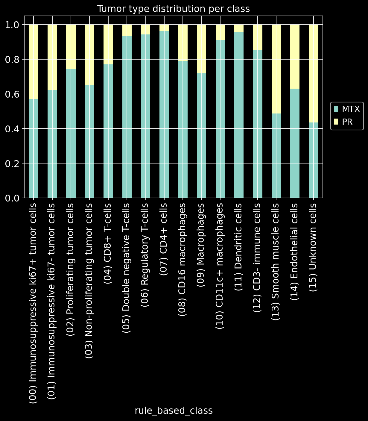
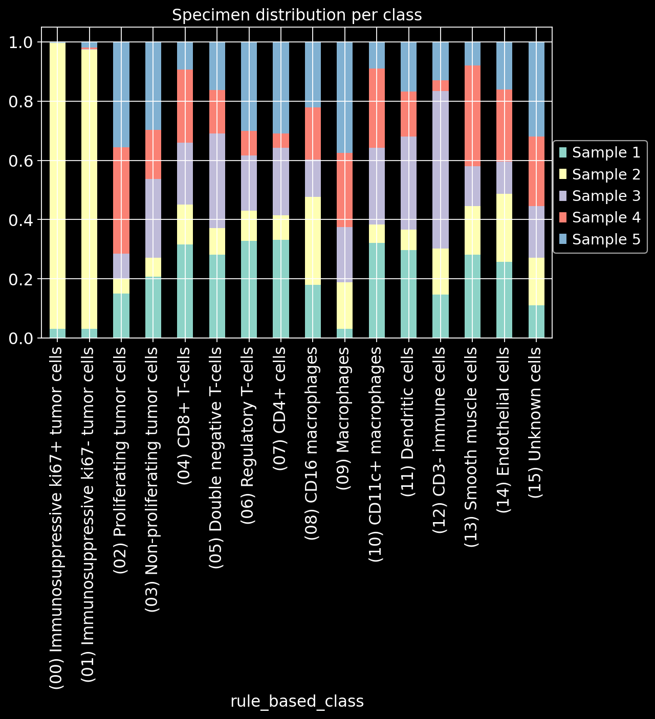
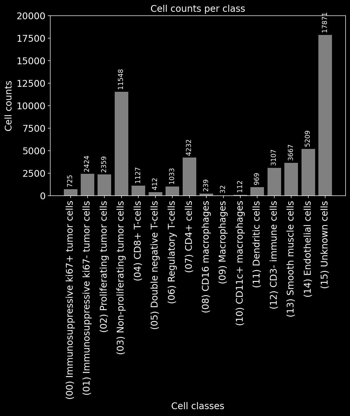
Plot distributions per tumor type, per sample and cell count bar plot

sc.set_figure_params(figsize='8,5')
plt.style.use('dark_background')
title_1 = 'Tumor type distribution per class'
title_2 = 'Specimen distribution per class'
tmp = pd.crosstab(adata_supervised.obs['rule_based_class'],adata_supervised.obs['type'], normalize = 'index') 
tmp.plot.bar(stacked=True, title = title_1).legend(loc='lower right',bbox_to_anchor=(1.15, 0.35))

tmp = pd.crosstab(adata_supervised.obs['rule_based_class'],adata_supervised.obs['samples'], normalize = 'index') 
tmp.plot.bar(stacked=True, title = title_2).legend(loc='lower right',bbox_to_anchor=(1.2, 0.25))

# Create a bar plot for counts
counts = adata_supervised.obs['rule_based_class'].value_counts().sort_index()
# Get data
categories = counts.index.to_numpy()
values = counts.to_numpy()
# Plot bar plot
fig, _ = plot_bar_chart(categories, values)
plt.show()

array([ True,  True,  True, ...,  True, False,  True], shape=(55066,))
# Get X,Y coords recenter
X_coords, Y_coords = recenter_cores(adata_supervised, core_names_arranged)

# Create mask for unknowns
umask = rule_based_classes_ints != 16

# Create a plot
fig, ax = plt.subplots(figsize = (16,8))

ax.scatter(X_coords[umask], Y_coords[umask], c = rule_based_classes_ints[umask], cmap = 'tab20b', s = 0.7, vmin=0, vmax=18)

ax.set_ylim(500,-3500)
ax.set_xlim(-500,4500)
ax.set_facecolor('white')
ax.set_aspect('equal')
ax.axis('off')
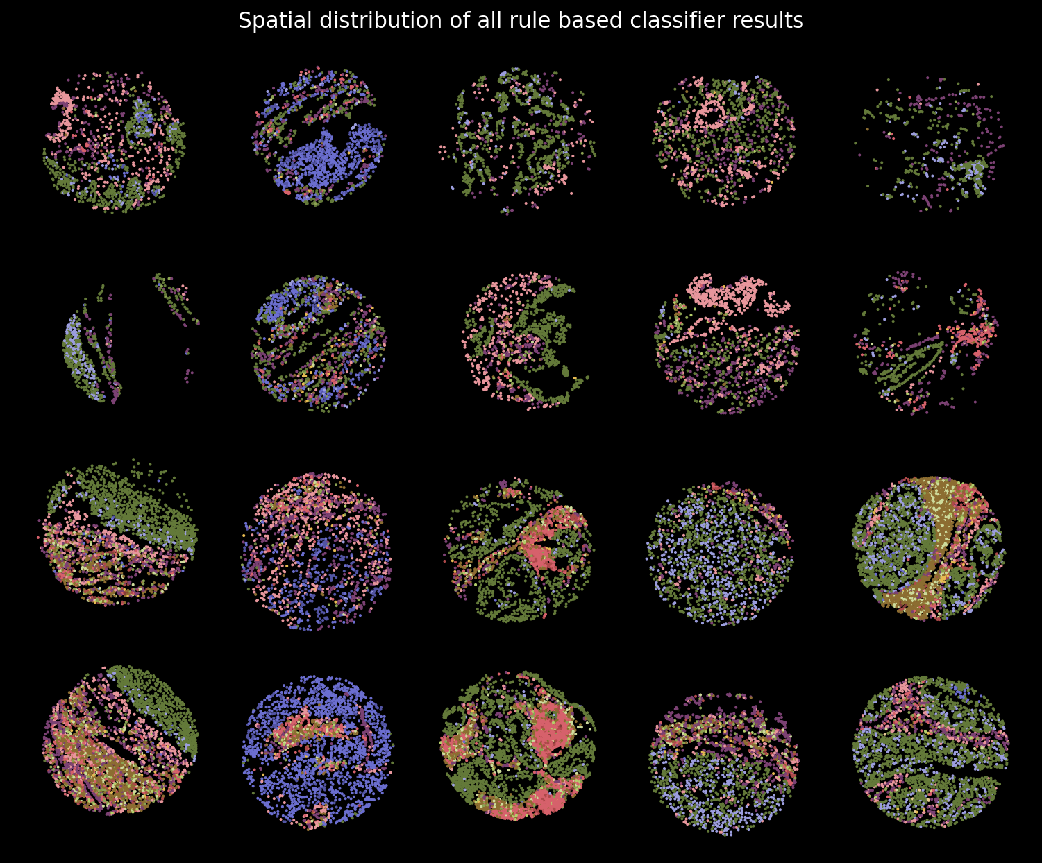
ax.set_title('Spatial distribution of all rule based classifier results')

plt.tight_layout()

Unsupervised phenotyping (Figure 4)

Perform Leiden clustering and UMAP on filtered data

The results of unsupervised clustering an dimensionality reduction using the provided version of scanpy dependency and its sub-dependencies are known to be computer dependent: https://github.com/scverse/scanpy/issues/2014


We provide the unsupervised clustering results that we obtained as a separate AnnData file.


If unsupervised clustring and UMAP is performed using RAW data, the final results are expected to be different and clsuter names need to be adjusted.


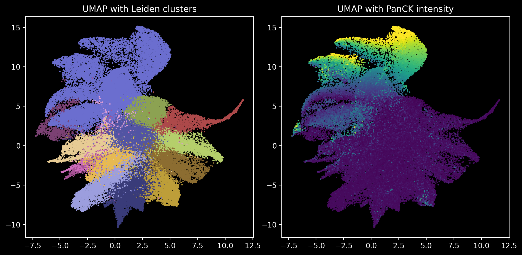
In subsequent steps the clusters on PanCK are merged into 1 metacluster and cluster 19 associated with false possitive segmentations is removed as described in the manuscript.

try:
    adata_unsupervised = anndata.read_h5ad('data/adata_unsupervised.h5ad')
except FileNotFoundError:
    print('Leiden clustering and UMAP will be performed locally. Results are likely to be different from original manuscript ')
    # Create an instance of anndata object
    adata_unsupervised = adata_phenotyping.copy()
    # Compute neighborhoods
    sc.pp.neighbors(adata_unsupervised, n_neighbors = 40)
    # Perform UMAP dimensionality reduction
    sc.tl.umap(adata_unsupervised, min_dist = 0.5)
    # Perform Leiden clustering
    sc.tl.leiden(adata_unsupervised, resolution = 0.8, key_added="RES=0.8")
adata_unsupervised
AnnData object with n_obs × n_vars = 55066 × 20
    obs: 'cores', 'type', 'samples', 'RES=0.8'
    uns: 'RES=0.8_colors', 'leiden', 'neighbors', 'umap'
    obsm: 'X_umap', 'spatial'
    obsp: 'connectivities', 'distances'
# Plot clustering results in UMAP coordinates
sc.set_figure_params(figsize='10,10')
plt.style.use('dark_background')
plt_name = 'UMAP Background subtracted and cleaned data'
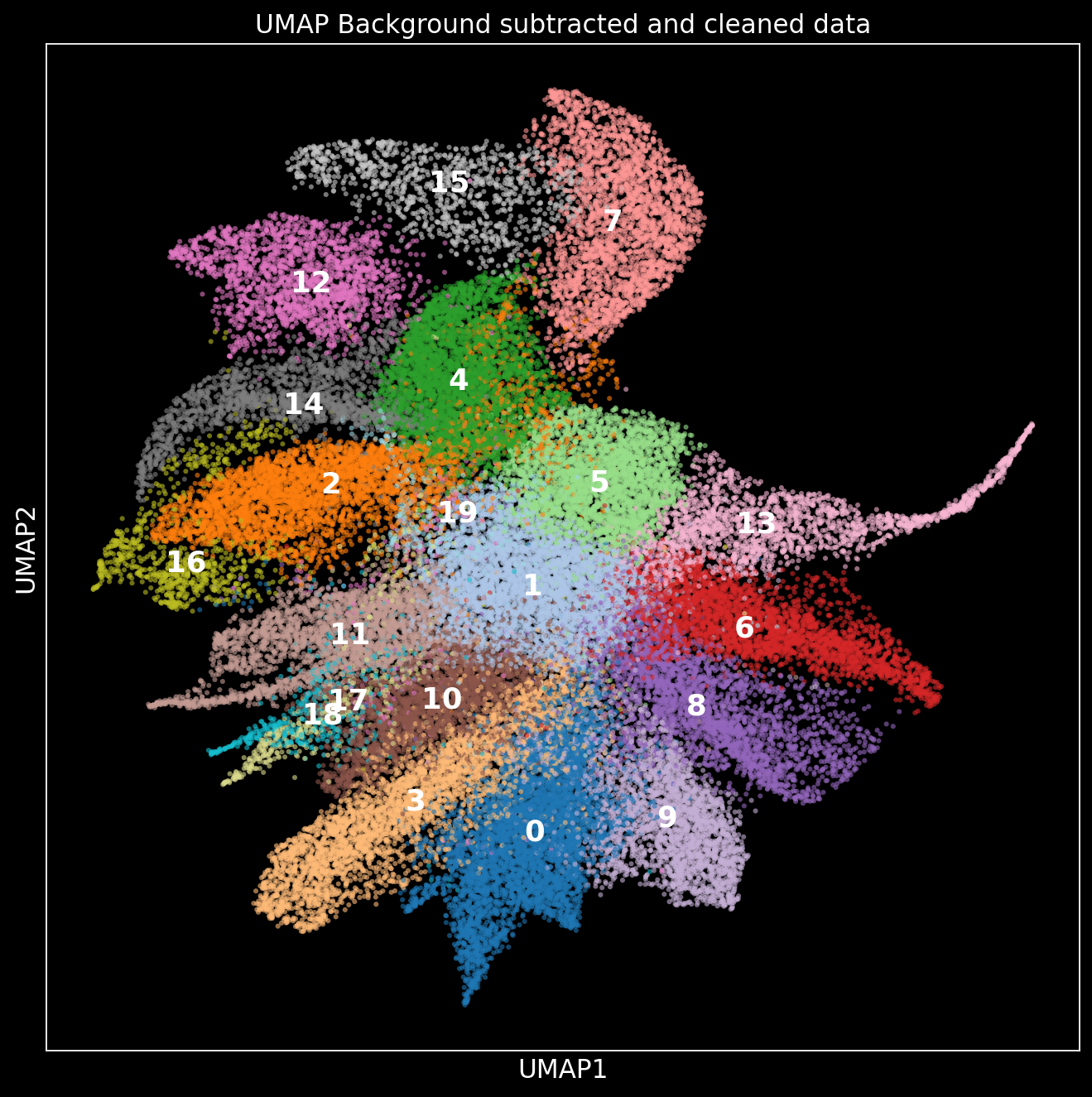
sc.pl.umap(adata_unsupervised, color="RES=0.8",  title = plt_name, palette = 'tab20', size = 30, alpha =  0.6, legend_loc = "on data", legend_fontsize = 16)

# Plot expression matrix
plt.style.use('default')
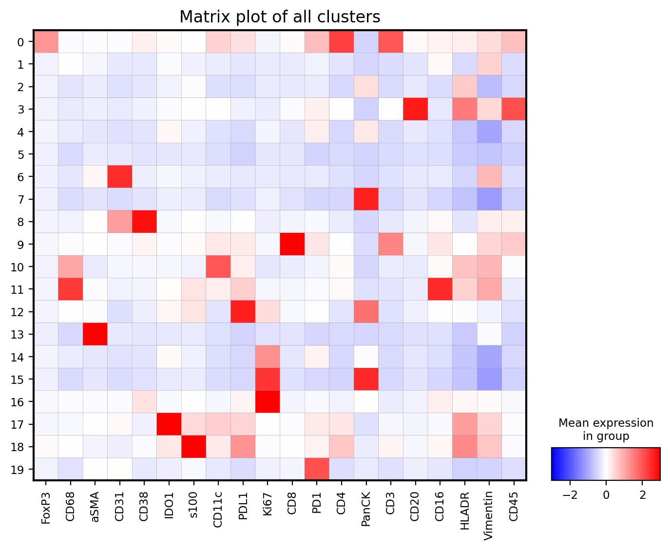
matrix_plot_name = 'Matrix plot of all clusters'
sc.pl.matrixplot(adata_unsupervised, title = matrix_plot_name, var_names = adata_unsupervised.var_names,groupby = 'RES=0.8', figsize = (8.3,6), cmap = 'bwr',  vmin = -3, vmax = 3)

Merge PanCK clusters

Idea here is to merge similar PanCK clusters into one metacluster for further analysis

help(merge_clusters)
Help on function merge_clusters in module utils.utils:

merge_clusters(cluster_arr: numpy.ndarray, clusters_to_merge: numpy.ndarray, new_name: str)
    Merge specified clusters in a cluster array or integers.
    
    Parameters:
        - cluster_arr (numpy.ndarray): Array of integers representing cluster names.
        - clusters_to_merge (numpy.ndarray): Array of integers specifying clusters to be merged.
        - new_name (str): New cluster name to assign to merged clusters.
    
    Returns:
        - numpy.ndarray: New cluster array with specified clusters merged.
# Visualize UMAP with cluster colors and UMAP with PanCK intensity
clusters = adata_unsupervised.obs_vector('RES=0.8').to_numpy(dtype = 'int')
UMAP_coords = adata_unsupervised.obsm['X_umap']
PancK_intensity = counts_markers_all.T[13]

# Merge Clusters
merged_clusters = merge_clusters(clusters, [2,4,7,12,15,14], 2)

plt.style.use('dark_background')
fig, (ax1, ax2) = plt.subplots(1, 2, figsize=(10, 5))
ax1.scatter(UMAP_coords[:, 0], UMAP_coords[:, 1], c = merged_clusters, s = 1, cmap = 'tab20b', label = merged_clusters)
ax1.set_title('UMAP with Leiden clusters')
ax2.scatter(UMAP_coords[:, 0], UMAP_coords[:, 1], c = PancK_intensity, s = 1, cmap = 'viridis', vmax = np.quantile(PancK_intensity, 0.99))
ax2.set_facecolor('black')
ax2.set_title('UMAP with PanCK intensity')
plt.tight_layout()

Remove cluster 19 and name each cluster with expected phenotype

len(filt_names) == adata_unsupervised_cleaned.n_obs
print(len(filt_names))
print(adata_unsupervised_cleaned.n_obs)
54583
55066
merged_clusters
print(np.unique(merged_clusters))
[ 0  1  2  3  5  6  8  9 10 11 13 16 17 18 19]
print(adata_unsupervised_cleaned.n_obs)
len(cluster_19_mask)
55066
55066
filt_names.astype('str')
array(['2', '2', '0', ..., '6', '8', '0'], shape=(54583,), dtype='<U21')
# Remove cluster 19 and create a new cleaned AnnData object.
# Create a mask for cluster 19
cluster_19_mask = merged_clusters != 19
# Filtered array of cluster names
filt_names = merged_clusters[cluster_19_mask].astype('int')
# Create a filtered AnnData object
adata_unsupervised_cleaned = adata_unsupervised.copy()
adata_unsupervised_cleaned = adata_unsupervised_cleaned[cluster_19_mask, :]


# Store cluster names as str in adata object
adata_unsupervised_cleaned.obs['Filtered clusters'] = filt_names.astype('str')
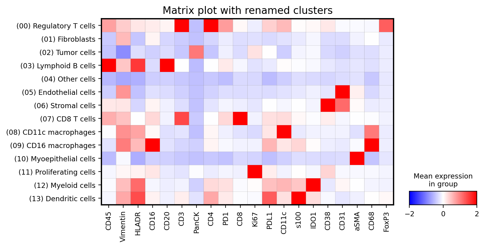
# Change the names based on the expression patterns
new_cluster_names = {
    0: '(00) Regulatory T cells',
    1: '(01) Fibroblasts',
    2: '(02) Tumor cells',
    3: '(03) Lymphoid B cells',
    5: '(04) Other cells',
    6: '(05) Endothelial cells',
    8: '(06) Stromal cells',
    9: '(07) CD8 T cells',
    10: '(08) CD11c macrophages',
    11: '(09) CD16 macrophages',
    13: '(10) Myoepithelial cells',
    16: '(11) Proliferating cells',
    17: '(12) Myeloid cells',
    18: '(13) Dendritic cells'}
full_names = [new_cluster_names.get(value, value) for value in filt_names]
adata_unsupervised_cleaned.obs['Renamed clusters'] = full_names
---------------------------------------------------------------------------
ValueError                                Traceback (most recent call last)
Cell In[116], line 13
      8 adata_unsupervised_cleaned = adata_unsupervised_cleaned[cluster_19_mask, :]
     12 # Store cluster names as str in adata object
---> 13 adata_unsupervised_cleaned.obs['Filtered clusters'] = filt_names.astype('str')
     14 # Change the names based on the expression patterns
     15 new_cluster_names = {
     16     0: '(00) Regulatory T cells',
     17     1: '(01) Fibroblasts',
   (...)     28     17: '(12) Myeloid cells',
     29     18: '(13) Dendritic cells'}

File ~/miniconda3/envs/squidpy/lib/python3.11/site-packages/anndata/_core/views.py:85, in _SetItemMixin.__setitem__(self, idx, value)
     78 else:
     79     warnings.warn(
     80         f"Trying to modify attribute `.{self._view_args.attrname}` of view, "
     81         "initializing view as actual.",
     82         ImplicitModificationWarning,
     83         stacklevel=2,
     84     )
---> 85     with view_update(*self._view_args) as container:
     86         container[idx] = value

File ~/miniconda3/envs/squidpy/lib/python3.11/contextlib.py:137, in _GeneratorContextManager.__enter__(self)
    135 del self.args, self.kwds, self.func
    136 try:
--> 137     return next(self.gen)
    138 except StopIteration:
    139     raise RuntimeError("generator didn't yield") from None

File ~/miniconda3/envs/squidpy/lib/python3.11/site-packages/anndata/_core/views.py:59, in view_update(adata_view, attr_name, keys)
     39 @contextmanager
     40 def view_update(adata_view: AnnData, attr_name: str, keys: tuple[str, ...]):
     41     """Context manager for updating a view of an AnnData object.
     42 
     43     Contains logic for "actualizing" a view. Yields the object to be modified in-place.
   (...)     57     `adata.attr[key1][key2][keyn]...`
     58     """
---> 59     new = adata_view.copy()
     60     attr = getattr(new, attr_name)
     61     container = reduce(lambda d, k: d[k], keys, attr)

File ~/miniconda3/envs/squidpy/lib/python3.11/site-packages/anndata/_core/anndata.py:1477, in AnnData.copy(self, filename)
   1471 if not self.isbacked:
   1472     if self.is_view and self._has_X():
   1473         # TODO: How do I unambiguously check if this is a copy?
   1474         # Subsetting this way means we don’t have to have a view type
   1475         # defined for the matrix, which is needed for some of the
   1476         # current distributed backend. Specifically Dask.
-> 1477         return self._mutated_copy(
   1478             X=_subset(self._adata_ref.X, (self._oidx, self._vidx)).copy()
   1479         )
   1480     else:
   1481         return self._mutated_copy()

File ~/miniconda3/envs/squidpy/lib/python3.11/site-packages/anndata/_core/anndata.py:1408, in AnnData._mutated_copy(self, **kwargs)
   1406         new[key] = kwargs[key]
   1407     else:
-> 1408         new[key] = getattr(self, key).copy()
   1409 if "X" in kwargs:
   1410     new["X"] = kwargs["X"]

File ~/miniconda3/envs/squidpy/lib/python3.11/site-packages/anndata/_core/aligned_mapping.py:125, in AlignedMappingBase.copy(self)
    123 def copy(self) -> dict[str, Value]:
    124     # Shallow copy for awkward array since their buffers are immutable
--> 125     return {
    126         k: copy(v) if isinstance(v, AwkArray) else v.copy() for k, v in self.items()
    127     }

File ~/miniconda3/envs/squidpy/lib/python3.11/site-packages/anndata/_core/aligned_mapping.py:125, in <dictcomp>(.0)
    123 def copy(self) -> dict[str, Value]:
    124     # Shallow copy for awkward array since their buffers are immutable
--> 125     return {
    126         k: copy(v) if isinstance(v, AwkArray) else v.copy() for k, v in self.items()
    127     }

File <frozen _collections_abc>:861, in __iter__(self)

File ~/miniconda3/envs/squidpy/lib/python3.11/site-packages/anndata/_core/aligned_mapping.py:164, in AlignedView.__getitem__(self, key)
    162 def __getitem__(self, key: str) -> Value:
    163     return as_view(
--> 164         _subset(self.parent_mapping[key], self.subset_idx),
    165         ElementRef(self.parent, self.attrname, (key,)),
    166     )

File ~/miniconda3/envs/squidpy/lib/python3.11/functools.py:909, in singledispatch.<locals>.wrapper(*args, **kw)
    905 if not args:
    906     raise TypeError(f'{funcname} requires at least '
    907                     '1 positional argument')
--> 909 return dispatch(args[0].__class__)(*args, **kw)

File ~/miniconda3/envs/squidpy/lib/python3.11/site-packages/anndata/_core/index.py:200, in _subset_sparse(a, subset_idx)
    198         first_idx = np.flatnonzero(first_idx)
    199     subset_idx = (first_idx.reshape(-1, 1), *subset_idx[1:])
--> 200 return a[subset_idx]

File ~/miniconda3/envs/squidpy/lib/python3.11/site-packages/scipy/sparse/_index.py:104, in IndexMixin.__getitem__(self, key)
    102             res = self.__class__(np.atleast_2d(row).shape, dtype=self.dtype)
    103         else:
--> 104             res = self._get_arrayXarray(row, col)
    106 # handle spmatrix (must be 2d, dont let 1d new_shape start reshape)
    107 if not isinstance(self, sparray):

File ~/miniconda3/envs/squidpy/lib/python3.11/site-packages/scipy/sparse/_compressed.py:565, in _cs_matrix._get_arrayXarray(self, row, col)
    562 minor = np.asarray(minor, dtype=idx_dtype)
    564 val = np.empty(major.size, dtype=self.dtype)
--> 565 csr_sample_values(M, N, self.indptr, self.indices, self.data,
    566                   major.size, major.ravel(), minor.ravel(), val)
    567 if major.ndim == 1:
    568     return self._ascontainer(val)

ValueError: could not convert integer scalar
Plot UMAP with Leiden clusters and a matrix plot

# Plot clustering results in UMAP coordinates
sc.set_figure_params(figsize='10,10')
plt.style.use('dark_background')
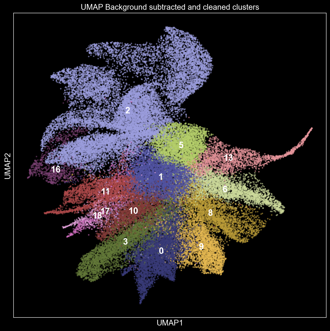
plt_name = 'UMAP Background subtracted and cleaned clusters'
sc.pl.umap(adata_unsupervised_cleaned, color="Filtered clusters", title = plt_name, palette = 'tab20b', size = 30, alpha =  0.6, legend_loc = "on data", legend_fontsize = 16)
... storing 'Filtered clusters' as categorical
... storing 'Renamed clusters' as categorical

# Plot expression matrix
plt.style.use('default')
matrix_plot_name = 'Matrix plot with renamed clusters'
sc.pl.matrixplot(adata_unsupervised_cleaned[::-1], title = matrix_plot_name, var_names = adata_unsupervised_cleaned.var_names[::-1],groupby = 'Renamed clusters', figsize = (8,4), cmap = 'bwr',  vmin = -2, vmax = 2)

Plot distributions per tumor type, per sample and cell count bar plot

sc.set_figure_params(figsize='8,5')
plt.style.use('dark_background')
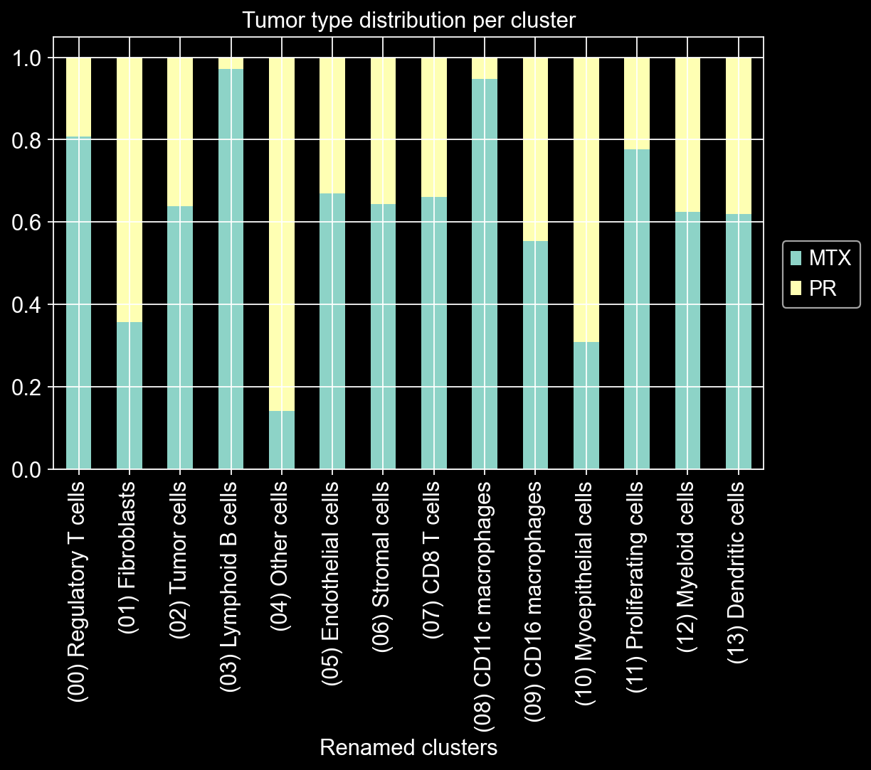
title_1 = 'Tumor type distribution per cluster'
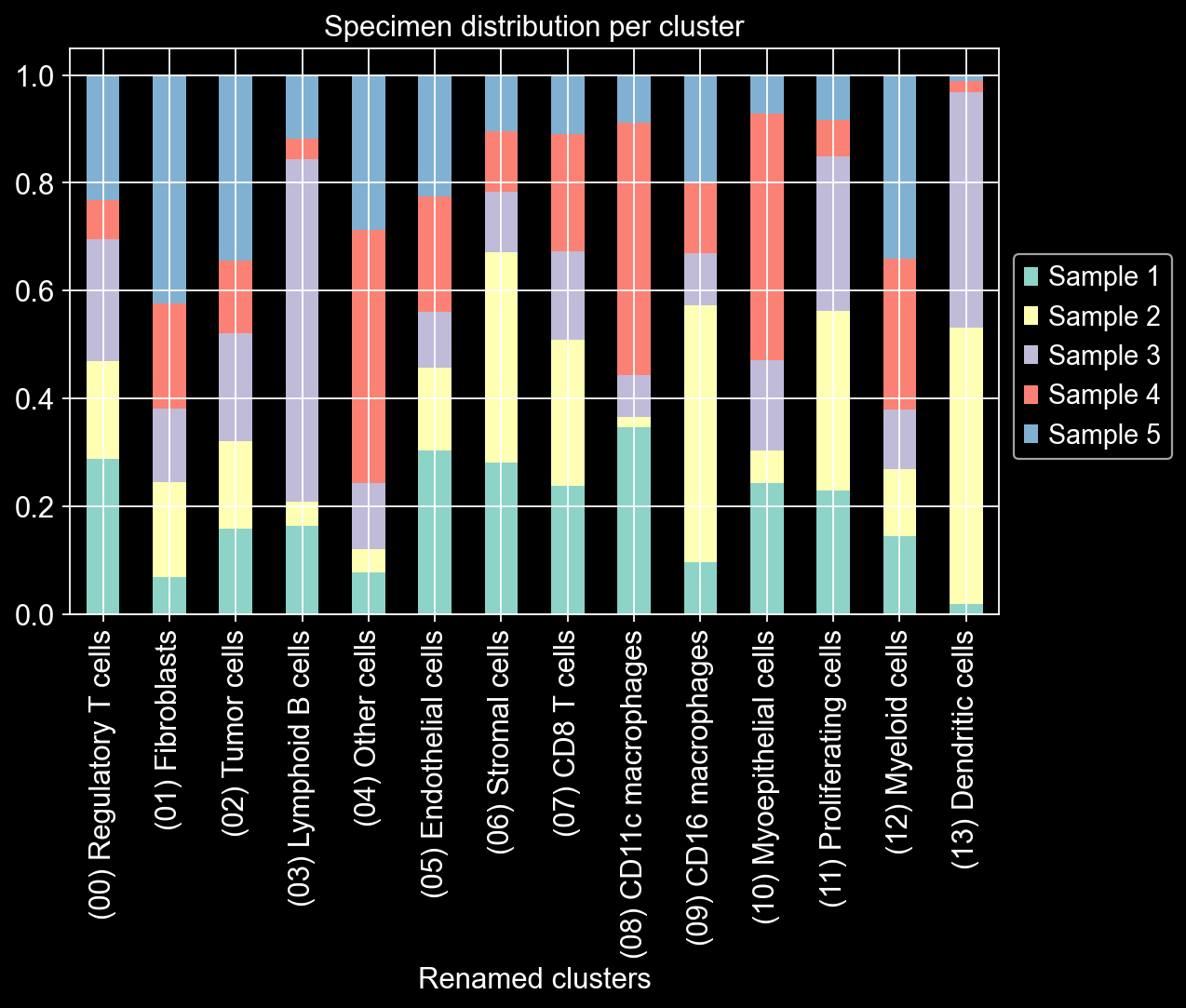
title_2 = 'Specimen distribution per cluster'
tmp = pd.crosstab(adata_unsupervised_cleaned.obs['Renamed clusters'],adata_unsupervised_cleaned.obs['type'], normalize = 'index') 
tmp.plot.bar(stacked=True, title = title_1).legend(loc='lower right',bbox_to_anchor=(1.15, 0.35))

tmp = pd.crosstab(adata_unsupervised_cleaned.obs['Renamed clusters'],adata_unsupervised_cleaned.obs['samples'], normalize = 'index') 
tmp.plot.bar(stacked=True, title = title_2).legend(loc='lower right',bbox_to_anchor=(1.2, 0.25))

# Create a bar plot for counts
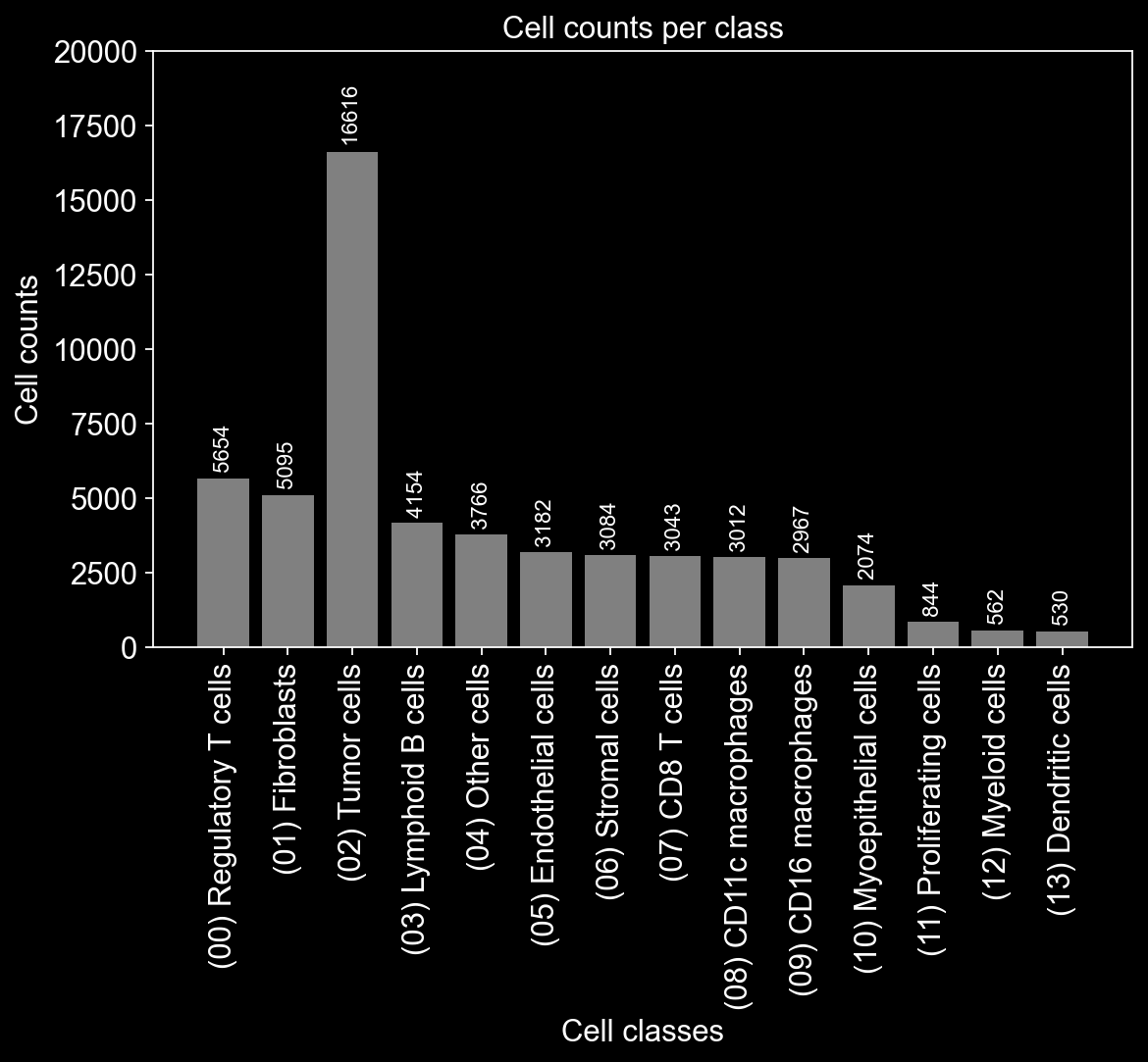
counts = adata_unsupervised_cleaned.obs['Renamed clusters'].value_counts().sort_index()
# Get data
categories = counts.index.to_numpy()
values = counts.to_numpy()
# Plot bar plot
fig, _ = plot_bar_chart(categories, values)
plt.show()

Plot clusters using spatial coordinates

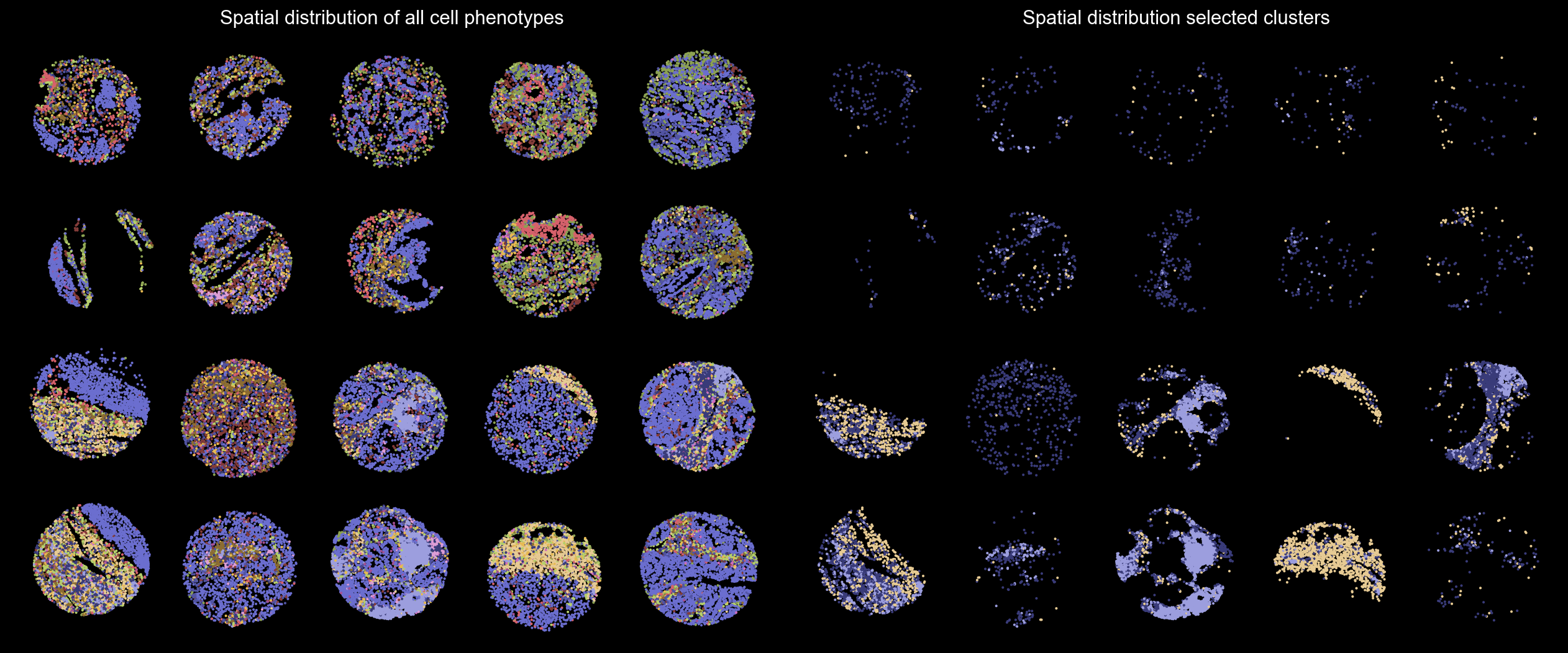
First each TMA core needs to be recentered and then the corresponding scatterplots will be made

# Get X,Y coords recenter
X_coords_uns, Y_coords_uns = recenter_cores(adata_unsupervised_cleaned, core_names_arranged)

# Get class names as integers
clusters_uns = adata_unsupervised_cleaned.obs['Filtered clusters'].to_numpy(dtype = 'int')
cluster_mask = np.isin(clusters_uns, [0,3,10])

# Create a plot
fig, (ax1, ax2) = plt.subplots(1, 2, figsize = (16,8))

ax1.scatter(X_coords_uns, Y_coords_uns, c = clusters_uns, cmap = 'tab20b', s = 0.7, vmin=0, vmax=18)
ax2.scatter(X_coords_uns[cluster_mask], Y_coords_uns[cluster_mask], c = clusters_uns[cluster_mask], cmap = 'tab20b', s = 0.7, vmin=0, vmax=18)

ax1.set_ylim(500,-3500); ax2.set_ylim(500,-3500)
ax1.set_xlim(-500,4500); ax2.set_xlim(-500,4500)

ax1.set_aspect('equal'); ax2.set_aspect('equal')
ax1.axis('off'); ax2.axis('off')

ax1.set_title('Spatial distribution of all cell phenotypes')
ax2.set_title('Spatial distribution selected clusters')

plt.tight_layout()

Make averaged cell images for specific class per each channel

try:
    # Make averaged images
    CK_av_image = make_averaged_crop(img_path=img_path,
                                    marker_name='PanCK',
                                    cluster_name='(02) Tumor cells',
                                    cluster_names=full_names,
                                    adata=adata_unsupervised_cleaned,
                                    img_px_size=px_size)

    CD3_av_image = make_averaged_crop(img_path=img_path,
                                    marker_name='CD3',
                                    cluster_name='(00) Regulatory T cells',
                                    cluster_names=full_names,
                                    adata=adata_unsupervised_cleaned,
                                    img_px_size=px_size)

    CD4_av_image = make_averaged_crop(img_path=img_path,  
                                    marker_name='CD4',
                                    cluster_name='(00) Regulatory T cells',
                                    cluster_names = full_names,
                                    adata=adata_unsupervised_cleaned,
                                    img_px_size=px_size)

    FoxP3_av_image = make_averaged_crop(img_path=img_path,
                                    marker_name='FoxP3',
                                    cluster_name='(00) Regulatory T cells',
                                    cluster_names = full_names,
                                    adata=adata_unsupervised_cleaned,
                                    img_px_size=px_size)
    
    # Plot all averaged images
    av_images = [CK_av_image, CD3_av_image, CD4_av_image, FoxP3_av_image]
    titles = ['PanCK', 'CD3', 'CD4', 'FoxP3']
    img_intensities = [[500, 15000], [2500, 5000], [2500, 5000],[1000, 4000]]

    # Create a figure with subplots
    fig, axs = plt.subplots(1, len(av_images), figsize=(15, 5))

     # Display each image with its title
    for ax, image, title, vmin_vmax in zip(axs, av_images, titles, img_intensities):
        im = ax.imshow(image, cmap='gray', vmin = vmin_vmax[0], vmax = vmin_vmax[1])  # Adjust the cmap based on your image type
        ax.set_title(title)
        cbar = plt.colorbar(im, ax=ax, orientation='horizontal', fraction=0.046, pad=0.04)  # Add color-bar
        ax.axis('off')  # Hide axes

    # Adjust layout and display the plot
    plt.tight_layout()
    fig.suptitle('Averaged marker images', fontsize = 20)
    plt.show()
except ValueError:
    print(f'Image in a specified path {img_path} was not found. Skipping this cell')
Image in a specified path data/TMA_downstream_analysis.ome.tiff was not found. Skipping this cell

Spatial analysis (Figure 5)

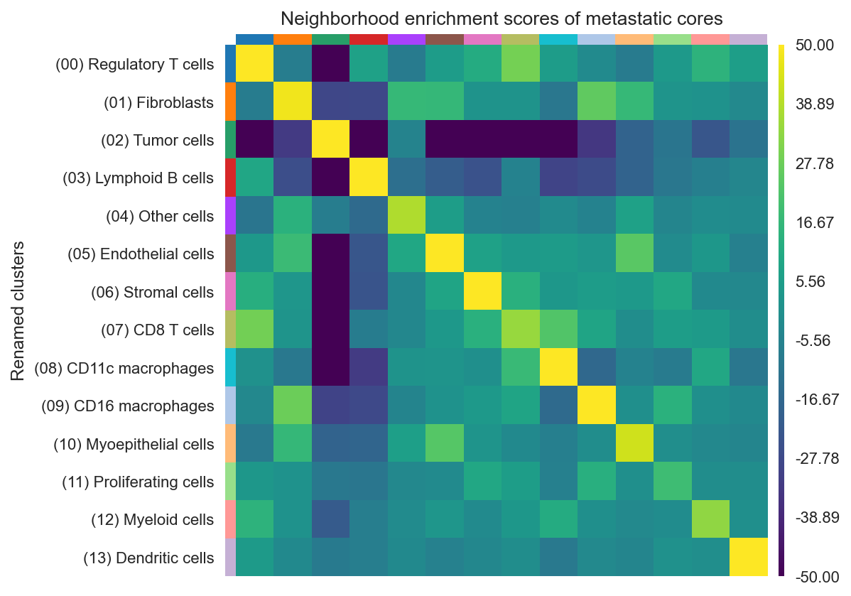
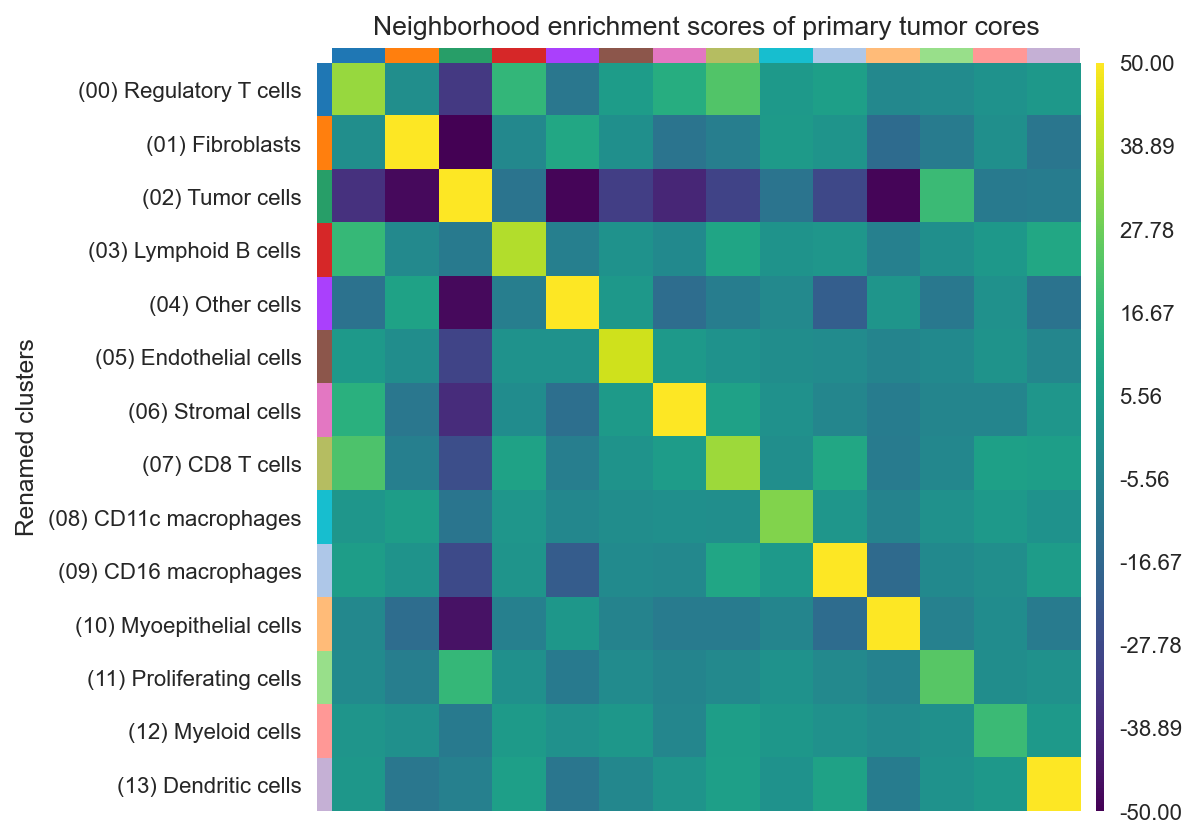
Here the Squidpy package is going to be used to create Neighborhood enrichment and interaction matrices

#Copy adata object
adata_spatial =adata_unsupervised_cleaned.copy()

filt_MTX = adata_spatial[adata_spatial.obs['type'] == 'MTX']
filt_PR = adata_spatial[adata_spatial.obs['type'] == 'PR']

#Calculate neighbors
sq.gr.spatial_neighbors(filt_MTX, coord_type="generic")
sq.gr.nhood_enrichment(filt_MTX, cluster_key="Renamed clusters")

sq.gr.spatial_neighbors(filt_PR, coord_type="generic")
sq.gr.nhood_enrichment(filt_PR, cluster_key="Renamed clusters")
100%|████████████████████████████████████████████████████████████████████████████████| 1000/1000 [00:12<00:00, 76.93/s]
100%|████████████████████████████████████████████████████████████████████████████████| 1000/1000 [00:10<00:00, 96.41/s]
sc.set_figure_params()
plt.style.use('seaborn')
plot_title = 'Neighborhood enrichment scores of metastatic cores'
sq.pl.nhood_enrichment(filt_MTX, figsize = (5,5), title = plot_title, cluster_key="Renamed clusters", cmap = 'viridis', mode = 'zscore', vmin=-50, vmax=50) 

sc.set_figure_params()
plt.style.use('seaborn')
plot_title = 'Neighborhood enrichment scores of primary tumor cores'
sq.pl.nhood_enrichment(filt_PR, title = plot_title, figsize = (5,5), cluster_key="Renamed clusters", cmap = 'viridis', mode = 'zscore', vmin=-50, vmax=50)

sc.set_figure_params()
plt.style.use('seaborn')
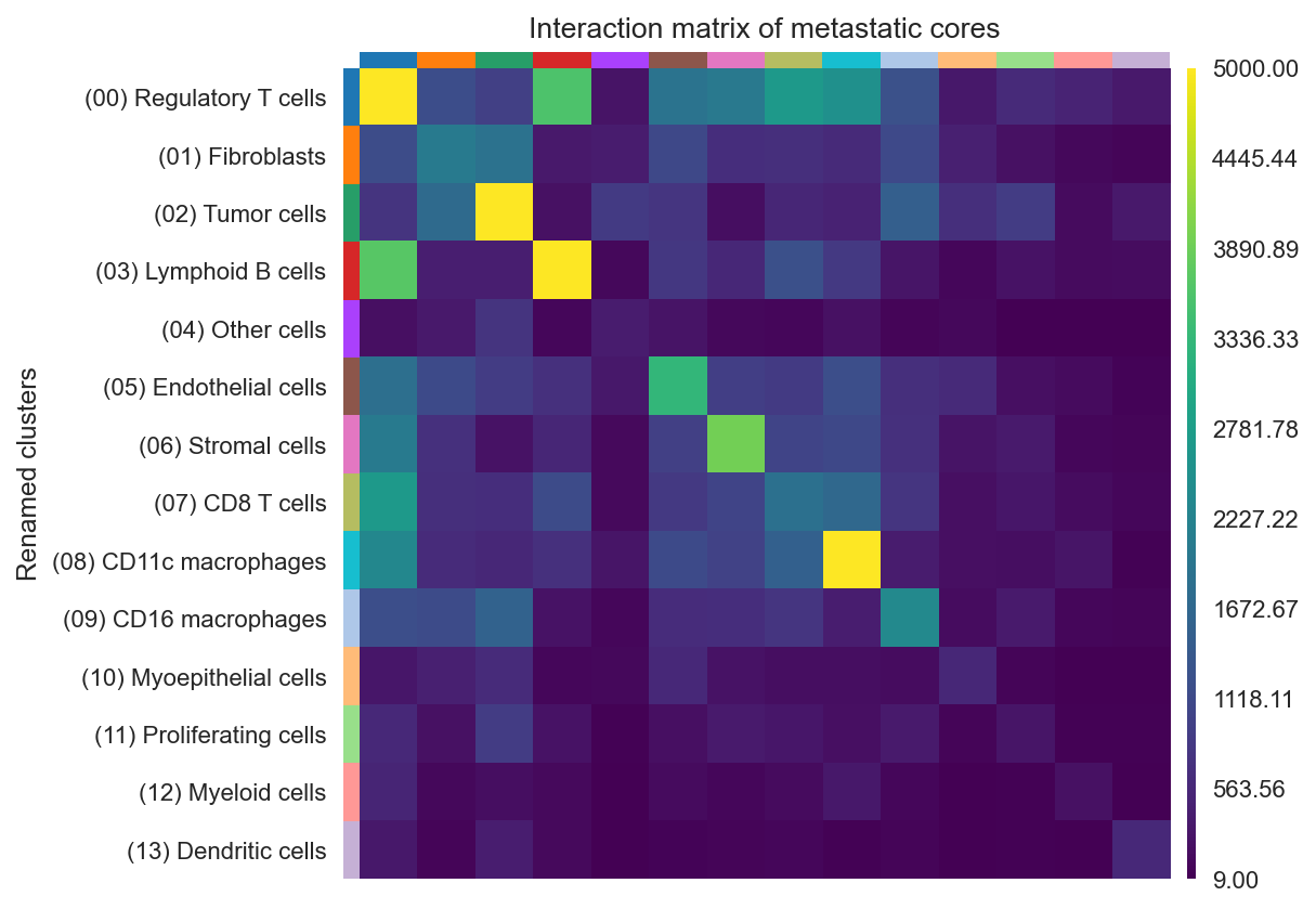
plot_title = 'Interaction matrix of metastatic cores'
sq.gr.interaction_matrix(filt_MTX, cluster_key="Renamed clusters")
sq.pl.interaction_matrix(filt_MTX, title = plot_title, figsize = (5,5), cluster_key="Renamed clusters", mode = 'zscore', vmax=5000) 

sc.set_figure_params()
plt.style.use('seaborn')
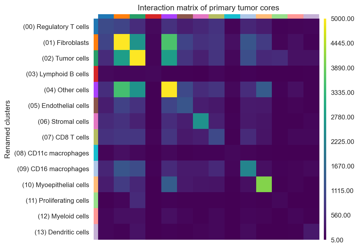
plot_title = 'Interaction matrix of primary tumor cores'
sq.gr.interaction_matrix(filt_PR, cluster_key="Renamed clusters")
sq.pl.interaction_matrix(filt_PR, title = plot_title, figsize = (5,5), cluster_key="Renamed clusters", mode = 'zscore', vmax=5000) 

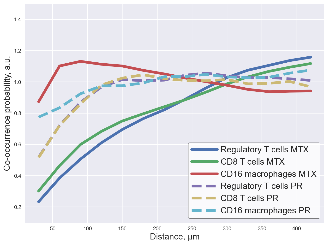
Co-occurrence scores

Calculate co-occurrence scores per core and then average the matching ones

    1. Filter based on metastatic and primary CORES
    1. Calculate co-ocurrence scores
    1. Average scores from each core
coo_intervals = np.arange(0,430,30)

MTX_coo_matrix = get_average_co_occurrence_matrix(filt_MTX,
                                                 coo_intervals,
                                                 cluster_obs_key='Renamed clusters',
                                                 cores_obs_key='cores')
PR_coo_matrix = get_average_co_occurrence_matrix(filt_PR,
                                                 coo_intervals,
                                                 cluster_obs_key='Renamed clusters',
                                                 cores_obs_key='cores')
100%|██████████████████████████████████████████████████████████████████████████████████| 10/10 [00:13<00:00,  1.38s/it]
100%|██████████████████████████████████████████████████████████████████████████████████| 10/10 [00:05<00:00,  1.85it/s]

Plot co-occurrence scores of interest

# Plot average co-occurrence scores
clust_CK = 2 # (02) Tumor cells
clust_T_reg = 0 # (00) Regulatory T cells
clust_CD16 = 9 # (09) CD16 macrophages
clust_CD8T = 7 # (07) CD8 T cells

index_to_cluster_name = {
    2: "Tumor cells",
    0: "Regulatory T cells",
    9: "CD16 macrophages",
    7: "CD8 T cells"
}

interval_crop = coo_intervals[0:-1]

fig = plt.figure(figsize = (10,7.5))
for s, subcluster in enumerate(MTX_coo_matrix[clust_CK]):
    if s == clust_CK:
        pass
    elif s == clust_CD16 or s == clust_T_reg or s == clust_CD8T:
        plt.plot(interval_crop+30, subcluster, label = str(index_to_cluster_name[s]) + ' MTX', lw = 5)
plt.legend(loc="upper center", mode = "expand", ncol = 10)


for s, subcluster in enumerate(PR_coo_matrix[clust_CK]):
    if s == clust_CK:
        pass
    elif s == clust_CD16 or s == clust_T_reg or s == clust_CD8T:
        plt.plot(interval_crop+30, subcluster, label = str(index_to_cluster_name[s])+' PR', lw = 5, linestyle = '--')

plt.legend(loc="lower right", handlelength = 3, fontsize = 16, frameon=True, facecolor='white', edgecolor='black')
plt.xlabel('Distance, \u00b5m', fontsize = 16)
plt.ylabel('Co-occurrence probability, a.u.', fontsize = 16)
plt.ylim(0.1, 1.5)
plt.show()